Write calculations to group and analyze your data.
In this series, we provide tips for how to effectively build a semantic model (formerly a dataset) in Power BI or Analysis Services. In the previous article, we described how you validate model relationships, which are links between tables and the foundation of your business logic. Once you’ve created and validated your relationships, you should now have the foundation of your model ready so that you can proceed with the next step.
In this article, we describe this next step in making a semantic model, where you create calculations by writing DAX. You reference the tables, columns, and relationships you’ve added to the model in previous steps to define these calculations for reports. These calculations are what you use in report visuals or Excel pivot tables to analyze your data.
The purpose of this article is to give an overview of the basics–when you write DAX, and how you can do this in Power BI Desktop, Tabular Editor or Microsoft Fabric.
- Semantic models in simple terms: what is a semantic model?
- Gather requirements for a semantic model.
- Prepare your data for a semantic model.
- Connect to and transform data for a semantic model.
- Create semantic model relationships.
- Validate semantic model relationships.
- DAX basics in a semantic model (this article).
What is DAX?
Data analysis expressions (DAX) is a functional and query programming language used in Power BI and other applications to analyse data. You write DAX expressions to define custom calculations or logic inside a model, and Power BI uses DAX queries to query the model from your report. DAX is how your visuals communicate with the semantic model to retrieve the data you need. The functional DAX you write are like instructions that tells the model which tables and columns to use, and what to do with them. When you write DAX, you reference tables, relationships, columns, and other calculations (measures), then use functions like SUM or AVERAGE to aggregate or filter data.
The following image shows the difference between a DAX expression and a DAX query. DAX queries are generated by Power BI to get data from a model, but advanced users might want to write DAX queries themselves for testing or validation purposes, or to automate certain tasks. We talk more about this in later articles of this series.
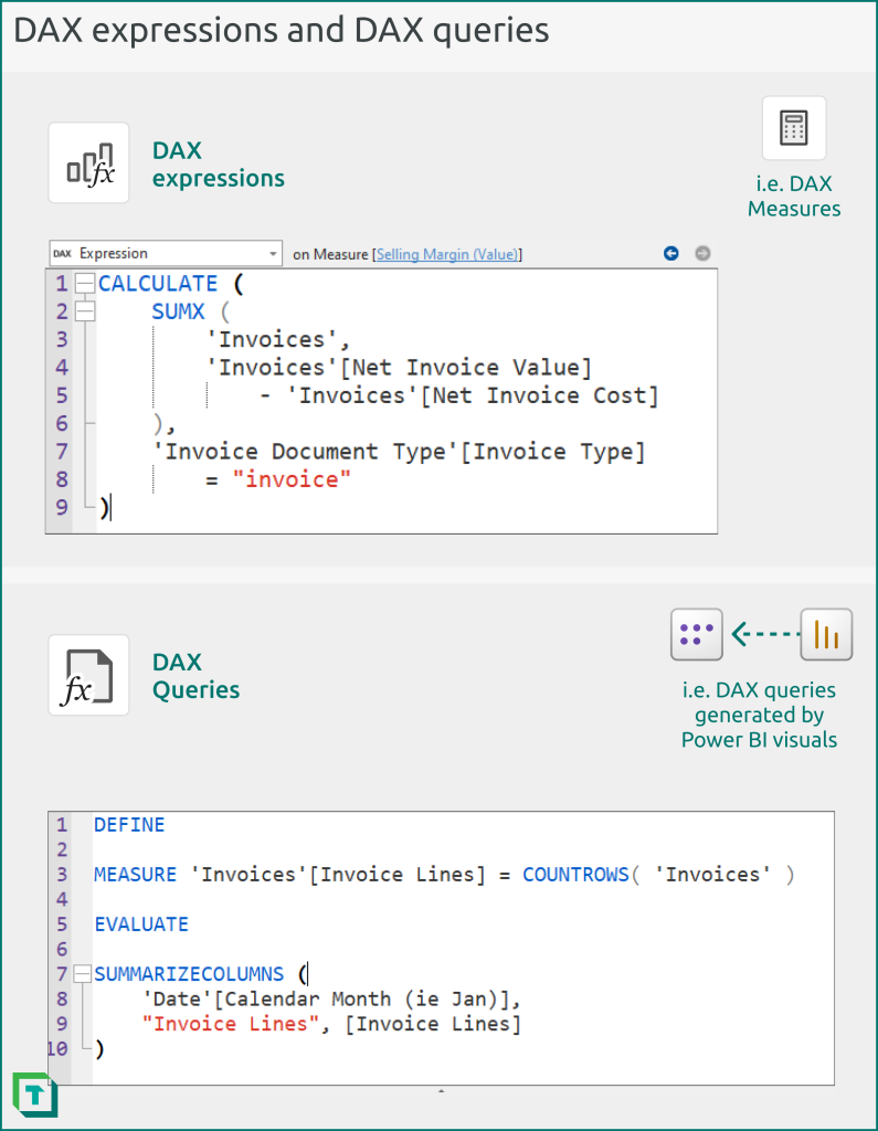
The previous example can be understood as follows:
- The first image shows a measure [Selling Margin (Value)]. It computes the sum of each row in the ‘Invoices’ table, subtracting the value in the ‘Invoices'[Net Invoice Cost] column from the value in the ‘Invoices'[Net Invoice Value] column. Since the selling margin should only be calculated for invoice documents (and not other document types), a CALCULATE function filters the result to only invoices by using the related ‘Invoice Document Type'[Invoice Type] column, which is a dimension table related to the ‘Invoices’ fact table. Measures are typically used in DAX queries, where they may produce different results based on which filters are currently active.
- The second image shows a DAX query for invoice lines by month. The query defines the measure [Invoice Lines] (which thus only exists in the query), and uses it in the query (after EVALUATE) to compute the lines by month. A developer might periodically run a query like this to validate the model or underlying data. A query can also refer to measures defined inside the model.
DAX occurs throughout a Power BI solution. The following image depicts a basic overview of the different places where you might write DAX in Power BI models and reports.
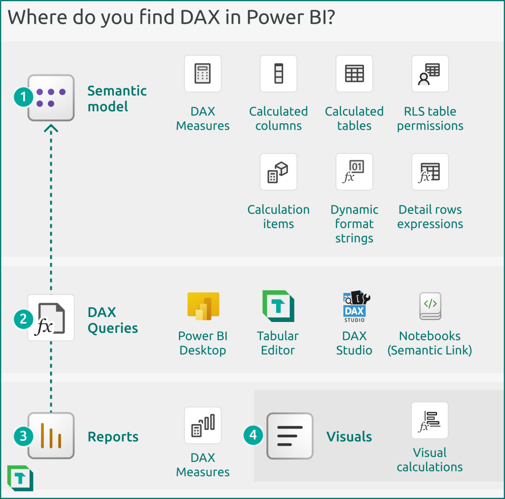
DAX exists throughout Power BI
- Semantic model: You write DAX in a model to define measures that you evaluate on-the-fly, or calculated tables and columns evaluated on model refresh. DAX expressions are also used to define row-level security (RLS) rules, called table permissions. DAX is also used on more advanced model objects, such as calculation group items, dynamic format strings and detail rows.
- Queries: DAX queries are how Power BI retrieves model data to populate visuals for reports. You can also write queries yourself in Power BI Desktop and other tools like Tabular Editor, DAX Studio, and Fabric notebooks with Semantic Link.
- Report: You can write DAX measures in “thin” reports that are connected to a published semantic model. This is usually only done for measures specific to that report, and not calculations (which are better to put in the model).
- Visuals: You can write a special type of DAX called visual calculations in Power BI visuals. Visual calculations are not part of the model, and only use the data in that visual to produce the calculation result.
“DAX is simple, but it’s not easy”
DAX is a simple language in its syntax and structure, but it’s well-known that DAX is not easy to learn. DAX resembles the simplicity of the Excel formula language at first glance, but this can be deceiving, as it’s more sophisticated to be able to address more scenarios than you’d encounter in Excel. Since DAX relies on a data model instead of cell positions on a worksheet, authors have to “think using the data model”, which is challenging for a novice to data modelling. The following are typical concepts that an experienced developer takes for granted, but a new developer must learn through experience:
- A model contains multiple tables that are connected by relationships.
- Filters propagate along relationships in a direction from one table to another.
- Attributes on the “One” side of a relationship chain can group values that are on the “Many” side.
An additional reason why DAX is challenging is because it operates differently from other programming languages. Some conventions in DAX are unique to DAX; it “thinks” in a unique way. This means that some developers with experience in other languages can apply conventions or practices that don’t work—or worse—they work but produce a suboptimal result.
- A Python example: You shouldn’t use a “loop” in DAX, like you’d use a for loop or while loop in Python.
- A SQL example: You shouldn’t perform conditional aggregation in DAX using IF/THEN, like you would with CASE/WHEN in SQL.
The following are additional examples of specific conventions or rules in DAX that are challenging to understand when you first start to write the DAX language.
- You modify calculations by using functions such as CALCULATE or CALCULATETABLE. With these functions, you provide two different arguments, filters (which filter the result) and CALCULATE modifiers (which change the behaviour of how these functions work).
- CALCULATE modifiers let you fine-tune the calculation result but require that you understand the intermediate result you’re modifying.
- Filters are actually tables, which is a concept that’s hard for new users to understand.
- DAX is evaluated in a context that defines the result. There are two main contexts to know when you write DAX: a filter context and a row context.
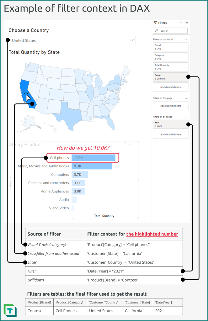
- A filter context filters the data. Examples of filter context include:
- When a filter or slicer is active in a report, or a user has applied filters in other ways like crossfiltering, drilldowns, or drillthroughs, and a DAX expression is evaluated in a visual of that report.
- When a DAX expression is evaluated for a specific data point in a visual (like a category or combination of categories).
- When a calculation provides a filter context as a CALCULATE argument (like ‘Date'[Month] = “January” ). This filter context overrides other filters on the referenced column, unless the KEEPFILTERS CALCULATE modifier is used.
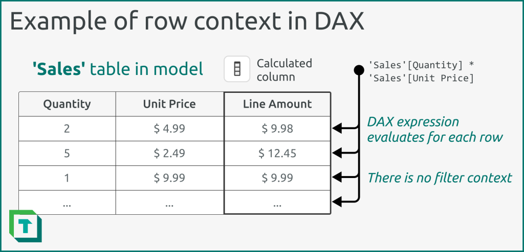
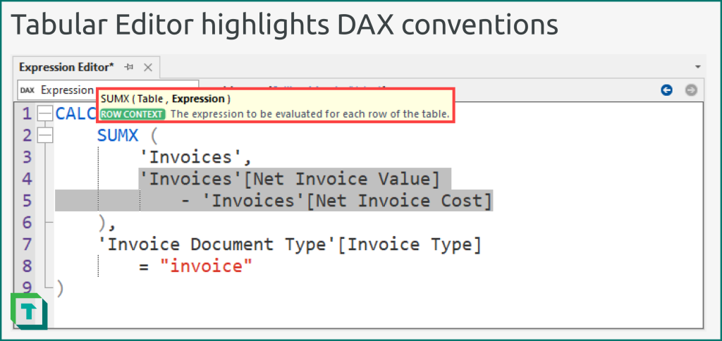
- A row context iterates tables. Examples of row context include:
- When you evaluate a DAX expression in a calculated column. For example, if you evaluate ‘Invoices’[Sales] – ‘Invoices’[Cost] in the ‘Invoices’ table in a calculated column, it uses a row context for the ‘Invoices’ table to get a result for each row.
- When you evaluate a DAX expression in an iterator function. For example, if you evaluate SUMX( ‘Invoices’, ‘Invoices’[Sales] – ‘Invoices’[Cost] ) in a DAX measure, it also uses the row context for the ‘Invoices’ table
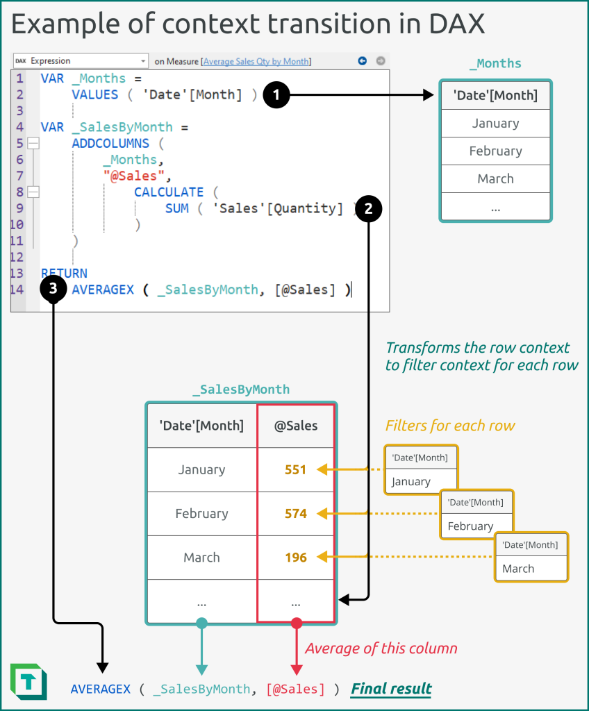
- The concept of context transition, which is when a row context is transformed into an equivalent filter context by using the CALCULATE function. Context transition can be a source of performance issues for many when they first start to write DAX.
Concepts like the above might sound intimidating, but don’t fear DAX; it’s very elegant and powerful. Despite what many LinkedIn influencers will tell you, you can benefit and get value from something without mastering it. For instance, in rare cases, you might not even need DAX in your semantic model.
Do I need to write DAX in my model?
You can create a model that has no DAX and use this data model to make a report. For instance, if you will only use the report to show data with descriptive attributes or unaggregated data, there’s no need to write any DAX. An example of this is a report for a product catalogue, or one designed to explore order documents by line item; raw transactions that aren’t summed together. However, reports like this are uncommon, since the benefit of Power BI reporting (and the VertiPaq engine that it uses) is to efficiently aggregate and visualize large, complex data.
You can also use implicit measures to analyse data without writing DAX.
Implicit measures
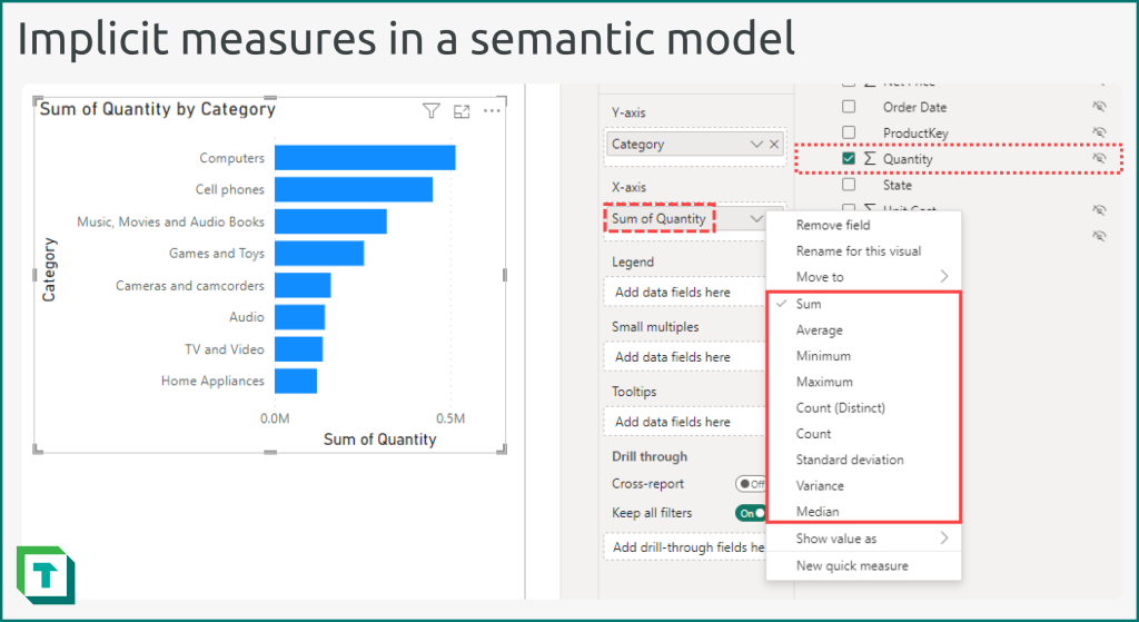
An implicit measure is what it’s called when you aggregate a numerical column in Power BI without writing any DAX. Instead, you add the column, and a default summarization is applied to group the data by a dimension. You can change this summarization from a set of default options. This is called implicit measure because behind the scenes, Power BI is creating the measure for you on-the-fly in the DAX query generated by the visual.
The following image depicts an example of an implicit measure Sum of Quantity from the Quantity column, grouped by the text column Category in the visual.
Implicit measures can be a good option for business users or people who are new to Power BI, particularly if they have no prior experience writing code. Additionally, even experienced developers might use implicit measures when doing a quick, ad hoc analysis (for instance when exploring data or analysing a short-lived model).
If you do plan to use implicit measures, consider the following points.
- Set the “Default Summarization” property to the appropriate aggregation. Set it to None for columns that shouldn’t be aggregated, like ‘Orders’[Order Number].
- Use display folders to organize numerical columns that can be aggregated away from other columns that cannot.
- Set a column description to clarify which aggregations should be used.
- Don’t use implicit measures if they aren’t going to provide a clear value. Particularly avoid using implicit measures of calculated columns, for instance, as a way of circumventing challenging DAX scenarios.
Implicit measures can be problematic and come with some caveats that you should be aware of.
- Options are limited to only the most frequently used aggregations.
- Since you can’t control the DAX, you have no ability to modify the calculation.
- Calculations don’t appear in the fields list, which makes it harder for a developer to understand how the model is being used or achieve consistency across reports.
- Adding calculation groups will discourage implicit measures in the model, meaning that users will be unable to create and use new implicit measures. Existing implicit measures in reports still work.
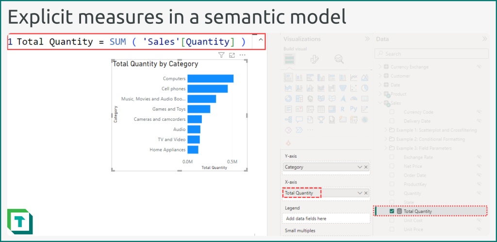
Explicit measures
While implicit measures have some valid use-cases, it’s generally preferred that you create explicit measures instead. Explicit measures are simply the DAX measures that you define yourself explicitly in the model (or in the connected “thin” report). The following example is the explicit measure version of the implicit measure from the previous image.
The following section describes more details about explicit DAX measures, and when you might use them instead of other DAX objects like calculated columns or tables.
Measures, Calculated Columns, and Calculated Tables
When you write DAX expressions, you do so in different object types: measures, calculated columns, or calculated tables.
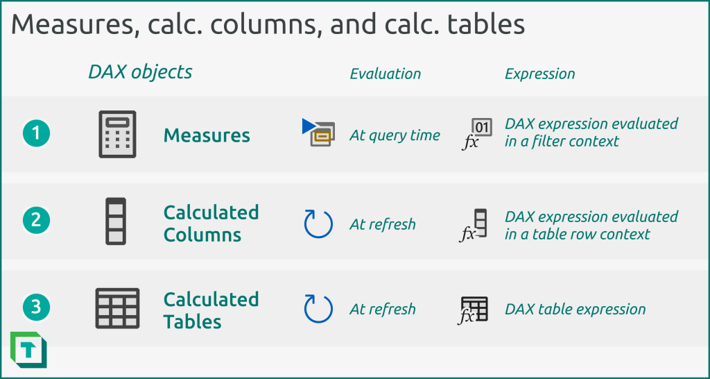
- Measures: Contains the definition of an expression (in DAX) and properties (like description, display folder, and format). A measure is simply metadata, and it’s associated with a table for organizational purposes. A measure is only evaluated when it’s queried (directly or by another measure that references it). An example of a measure is a Sales Amount measure that computes the SUM of all sales.
- Calculated columns: Contains a definition of an expression (in DAX) and properties (like description, data type, and format), as well as the data result. This data result of a calculated column makes your model consume more memory. Calculated columns are created in a table and evaluate the DAX for each row of the table. They are only evaluated when refreshed. An example of a calculated column could be a flag that identifies new customers with sales in the current month, which you use in other calculations.
- Calculated tables: Like a calculated column but evaluated independently of any existing tables and columns aside from the ones referenced in its DAX expression. A calculated table produces a stand-alone result of one or more columns. Like a calculated column, it’s also only evaluated when refreshed. An example of a calculated table could be a date table that you create with the CALENDAR DAX function.
- You will use the computed result as an attribute to group other calculations. An example is when you want to show sales in bins for a histogram visual.
- You will use the computed result to filter data. An example is when you want to dynamically “flag” certain transactions to filter out of another calculation or report.
- Generally, if you do need a calculated column, you should consider the potential benefits of pushing the calculation upstream to Power Query or further to the data source. However, for some scenarios, calculated columns are a perfectly valid approach. Examples might be:
- The tables are small, the calculations are simple, and you will add only a few.
- The model is developed by a self-service user with limited knowledge in Power Query and no upstream source system (i.e. Power BI connects to Excel files on a SharePoint or OneDrive).
- The calculation relies on other, dynamic data or attributes in the model.
Depending on the type of model you are making, you might not be able to create calculated columns or tables. If you have specific use-cases that require one of these objects, this might motivate your decision to use one storage mode or another.
The following figure gives an overview of which DAX objects you can create in the different semantic model storage modes available in Power BI, today.

In summary, the following restrictions apply to some types of semantic models. Note that the storage mode is set per table, except for Direct Lake, which doesn’t support combining tables of different storage modes (the entire model uses Direct Lake storage mode).
- Import: Models that import the data in-memory are the default (and most common) storage mode. You can create any DAX objects in these models.
- DirectQuery: Models that connect directly to a supported data source, converting DAX queries on-the-fly to equivalent SQL queries. These models don’t support calculated columns or tables.
- Hybrid: Models that have a mix of storage modes or hybrid tables don’t allow calculated columns in DirectQuery or Hybrid tables in the model.
- Direct Lake: Models that connect to Delta tables in a Fabric Lakehouse or Data Warehouse don’t support calculated columns, and only support calculated tables if they don’t reference Direct Lake tables, or columns from these tables. Direct Lake is only available if you have a Fabric capacity, and if you have the data available in OneLake data items as Delta tables.
In Conclusion
DAX is a fundamental part of most semantic models. It is a simple and powerful language, though it does have a few complex concepts that require a theoretical understanding to use most effectively. You use either DAX expressions or queries with your semantic model in different parts of your Power BI solution. In the next article, we provide tips and guidance about how you can effectively write DAX in your Power BI semantic models.

- Semantic models in simple terms: what is a semantic model?
- Gather requirements for a semantic model.
- Prepare your data for a semantic model.
- Connect to and transform data for a semantic model.
- Create semantic model relationships.
- Validate semantic model relationships.
- DAX basics in a semantic model (this article).